梳理 Human Parsing(人体解析) 相关介绍，数据集，算法

Intro

Foreword

人体解析(Human Parsing)是细粒度的语义分割任务，旨在识别像素级别的人类图像的组成部分（例如，身体部位和服装）。

What is Human Parsing

different from pedestrian segmentation
- 行人分割任务关注从图中抠出像素级的行人，目标可以是单人或者多人，往往是多人
- 人体解析关注将身体各部分像素级抠出，目标往往是单人
semantic understanding of person
- 像素级理解人体
mul-label segmentation track
- 是多类别分割任务

Usage of Human Parsing

pedestrian attribution
- more precising than label learning when using as a front method of pedestrian attribute learning
- 现在行人属性学习有两种主思路
  - mul-label learning
    - 使用标签对全图直接进行分类，使用attention进行unsupervised learning
    - 优点：打标成本低，方便大规模使用
    - 缺点：可靠性有待商榷
  - mul-task learning
    - 使用人体解析作为前置，扣出后进行分析
    - 优点：可靠，后续操作灵活，且自带粗略属性
    - 缺点：打标成本极高
Clothing Recommend
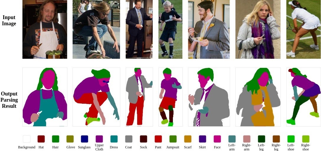
- Human Parsing 能够扣出
  -Hat
  -Hair
  -Glove
  -Sunglasses
  -Upper-clothes
  -Dress
  -Coat
  -Socks
  -Pants
  -Jumpsuits
  -Scarf
  -Skirt
- 在这个任务的基础上服饰的进一步解析推荐都是可期的
pose estimation
- human parsing 能够扣出
  - Face
  - Left-arm
  - Right-arm
  - Left-leg
  - Right-leg
  - Left-shoe
  - Right-shoe
- 理论上是可以拿来做pose estimation和single frame的action recognition
- 有些数据集例如 LIP 同时拥有人体关键点和人体解析的标注，联合优化目前做的人不多，理论上可行，有待研究
Re-ID
- 使用 human parsing 做对其然后进行re-id
- 有人这么玩过效果不错但是消耗资源大，成本也高

Algorithm

JPPNet

paper Look into Person: Joint Body Parsing & Pose Estimation Network and A New Benchmark
github https://github.com/Engineering-Course/LIP_JPPNet
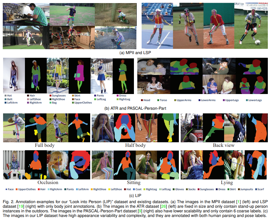
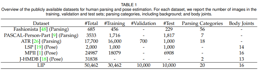
本文提出了重量级的 human parsing benchmark — LIP
从数据集内容丰富度上看，之前的数据集中，MPII 和 LSP 就只有线，ATR就站着的，Pascaljiu 6种标，而LIP啥都有
从数据集本身数量上看， LIP也领先其他数据集许多
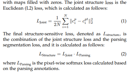
文章中提出了两种结构 JPPNet 以及没有pose帮助的 SS-JPPNet，来看主结构

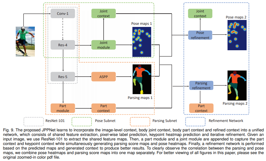
主要思想就是，共享backbone，fuse结果进行refine，具体是如何做的呢

#backbone中提取对应特征 
resnet_fea_100 = net_100.layers['res4b22_relu']
parsing_fea1_100 = net_100.layers['res5d_branch2b_parsing']
parsing_out1_100 = net_100.layers['fc1_human']

#backbone中提取对应特征 
resnet_fea_100 = net_100.layers['res4b22_relu']
parsing_fea1_100 = net_100.layers['res5d_branch2b_parsing']
parsing_out1_100 = net_100.layers['fc1_human']
    
#fc1_human是ASPP的output，出未refine的parsing结果。下面是源代码，是tf1.*的写法
(self.feed('res5b_relu','bn5c_branch2c')
.add(name='res5c')
.relu(name='res5c_relu')
.atrous_conv(3, 3, n_classes, 6, padding='SAME', relu=False, name='fc1_human_c0'))
    
(self.feed('res5c_relu')
.atrous_conv(3, 3, n_classes, 12, padding='SAME', relu=False, name='fc1_human_c1'))

(self.feed('res5c_relu')
.atrous_conv(3, 3, n_classes, 18, padding='SAME', relu=False, name='fc1_human_c2'))

(self.feed('res5c_relu')
.atrous_conv(3, 3, n_classes, 24, padding='SAME', relu=False, name='fc1_human_c3'))
 
(self.feed('fc1_human_c0',
'fc1_human_c1',
'fc1_human_c2',
'fc1_human_c3')
.add(name='fc1_human'))
 
#再结合posenet进行refine
def pose_net(image, name):
    with tf.variable_scope(name) as scope:
        is_BN = False
        pose_conv1 = conv2d(image, 512, 3, 1, relu=True, bn=is_BN, name='pose_conv1')
        pose_conv2 = conv2d(pose_conv1, 512, 3, 1, relu=True, bn=is_BN, name='pose_conv2')
        pose_conv3 = conv2d(pose_conv2, 256, 3, 1, relu=True, bn=is_BN, name='pose_conv3')
        pose_conv4 = conv2d(pose_conv3, 256, 3, 1, relu=True, bn=is_BN, name='pose_conv4')
        pose_conv5 = conv2d(pose_conv4, 256, 3, 1, relu=True, bn=is_BN, name='pose_conv5')
        pose_conv6 = conv2d(pose_conv5, 256, 3, 1, relu=True, bn=is_BN, name='pose_conv6')
    
        pose_conv7 = conv2d(pose_conv6, 512, 1, 1, relu=True, bn=is_BN, name='pose_conv7')
        pose_conv8 = conv2d(pose_conv7, 16, 1, 1, relu=False, bn=is_BN, name='pose_conv8')
    
        return pose_conv8, pose_conv6   #FCN结果，context
    
def pose_refine(pose, parsing, pose_fea, name):
    with tf.variable_scope(name) as scope:
        is_BN = False
        # 1*1 convolution remaps the heatmaps to match the number of channels of the intermediate features.
        pose = conv2d(pose, 128, 1, 1, relu=True, bn=is_BN, name='pose_remap')
        parsing = conv2d(parsing, 128, 1, 1, relu=True, bn=is_BN, name='parsing_remap')
        # concat 
        pos_par = tf.concat([pose, parsing, pose_fea], 3)
        conv1 = conv2d(pos_par, 512, 3, 1, relu=True, bn=is_BN, name='conv1')
        conv2 = conv2d(conv1, 256, 5, 1, relu=True, bn=is_BN, name='conv2')
        conv3 = conv2d(conv2, 256, 7, 1, relu=True, bn=is_BN, name='conv3')
        conv4 = conv2d(conv3, 256, 9, 1, relu=True, bn=is_BN, name='conv4')
        conv5 = conv2d(conv4, 256, 1, 1, relu=True, bn=is_BN, name='conv5')
        conv6 = conv2d(conv5, 16, 1, 1, relu=False, bn=is_BN, name='conv6')
        
        return conv6, conv4 #FCN结果，context

def parsing_refine(parsing, pose, parsing_fea, name):
    with tf.variable_scope(name) as scope:
        is_BN = False
        pose = conv2d(pose, 128, 1, 1, relu=True, bn=is_BN, name='pose_remap')
        parsing = conv2d(parsing, 128, 1, 1, relu=True, bn=is_BN, name='parsing_remap')
      
        par_pos = tf.concat([parsing, pose, parsing_fea], 3)
        parsing_conv1 = conv2d(par_pos, 512, 3, 1, relu=True, bn=is_BN, name='parsing_conv1')
        parsing_conv2 = conv2d(parsing_conv1, 256, 5, 1, relu=True, bn=is_BN, name='parsing_conv2')
        parsing_conv3 = conv2d(parsing_conv2, 256, 7, 1, relu=True, bn=is_BN, name='parsing_conv3')
        parsing_conv4 = conv2d(parsing_conv3, 256, 9, 1, relu=True, bn=is_BN, name='parsing_conv4')
      
        parsing_conv5 = conv2d(parsing_conv4, 256, 1, 1, relu=True, bn=is_BN, name='parsing_conv5')
        parsing_human1 = atrous_conv2d(parsing_conv5, 20, 3, rate=6, relu=False, name='parsing_human1')
        parsing_human2 = atrous_conv2d(parsing_conv5, 20, 3, rate=12, relu=False, name='parsing_human2')
        parsing_human3 = atrous_conv2d(parsing_conv5, 20, 3, rate=18, relu=False, name='parsing_human3')
        parsing_human4 = atrous_conv2d(parsing_conv5, 20, 3, rate=24, relu=False, name='parsing_human4')
        parsing_human = tf.add_n([parsing_human1, parsing_human2, parsing_human3, parsing_human4], name='parsing_human')
            
        return parsing_human, parsing_conv4 #FCN结果，context

总体来说分以下几个步骤
1. pose_out1_100, pose_fea1_100 = pose_net(resnet_fea_100, ‘fc1_pose’) #先出一次pose结果
2. pose_out2_100, pose_fea2_100 = pose_refine(pose_out1_100, parsing_out1_100, pose_fea1_100, name=’fc2_pose’) # 结合第一次parsing结果出第二次pose结果
3. parsing_out2_100, parsing_fea2_100 = parsing_refine( parsing_out1_100, pose_out1_100, parsing_fea1_100, name=’fc2_parsing’) # 结合第一次pose结果出第二次parsing结果
4. parsing_out3_100, parsing_fea3_100 = parsing_refine(parsing_out2_100, pose_out2_100, parsing_fea2_100, name=’fc3_parsing’) # 结合第二次pose结果出第三次parsing结果
5. pose_out3_100, pose_fea3_100 = pose_refine(pose_out2_100, parsing_out2_100, pose_fea2_100, name=’fc3_pose’) # 结合第二次parsing结果出第三次pose结果
从代码上看，和论文里的图略有不同
loss
experiment
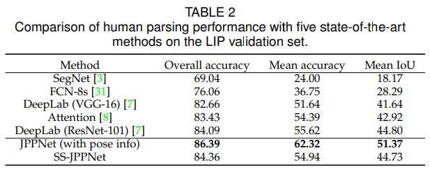
- 从实验结果上看效果提升很明显，值得一赞
more
- 值得一提的是，SS-JPPNet 咋就和DeepLab差不多呢？上图
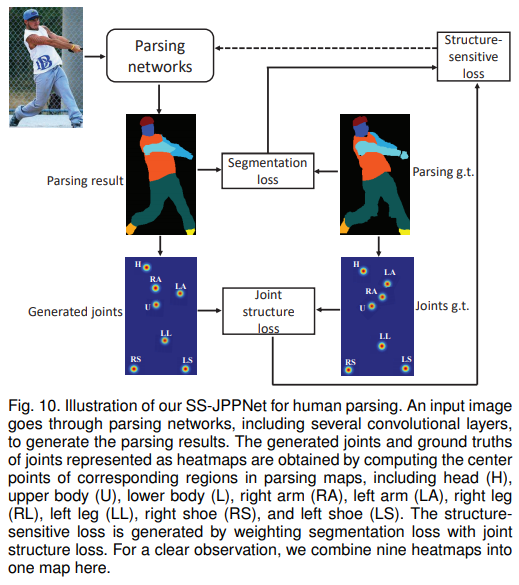
- 通过human parsing的9个部位，取其中心作为关键点进行训练，结果也是意料之中的没什么卵用。猜测是关键点结果还是来自于human parsing的结果，监督信息耦合。结果也是和deeplab相近

CE2P

paper Devil in the Details: Towards Accurate Single and Multiple Human Parsing
github https://github.com/liutinglt/CE2P
参考链接 https://blog.csdn.net/siyue0211/article/details/90927712
标题很风骚，内容还是很硬核的
人体解析现在主要有两大类解决方案：
1. High-resolution Maintenance，这种方法通过获得高分辨率的特征来恢复细节信息。它存在的问题是，由于卷积中的池化操作和卷积中的步长，会让最终生成的特征较小。解决方法是，删除一些下采样操作（max pooling etc.）或从一些低层特征中获取信息。
2. Context Information Embedding. 这种方法通过捕获丰富的上下文信息来处理多尺度的对象。ASPP和PSP是使用这一方式解决问题的主要结构。
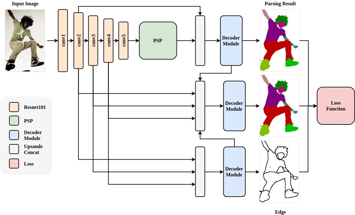
CE2P主要包括三大模块：
1. 一个高分辨率的embedding 模块，作用是放大特征图以恢复细节
2. 一个全局上下文embedding 模块，作用是编码多尺度的上下文信息
3. 一个边缘感知模块，用于整合对象轮廓的特征，以细化解析预测的边界
Contribution
1. 作者分析了一些人脸解析方法，验证其有效性。并说明如何使用这些方法来达到更好的效果
2. 作者利用了人脸解析中一些有效的方法，构建了CE2P框架
3. CE2P框架达到了公开数据集state-of-art的效果
4. 代码开源，可以作为baseline使用

下面来看看结构

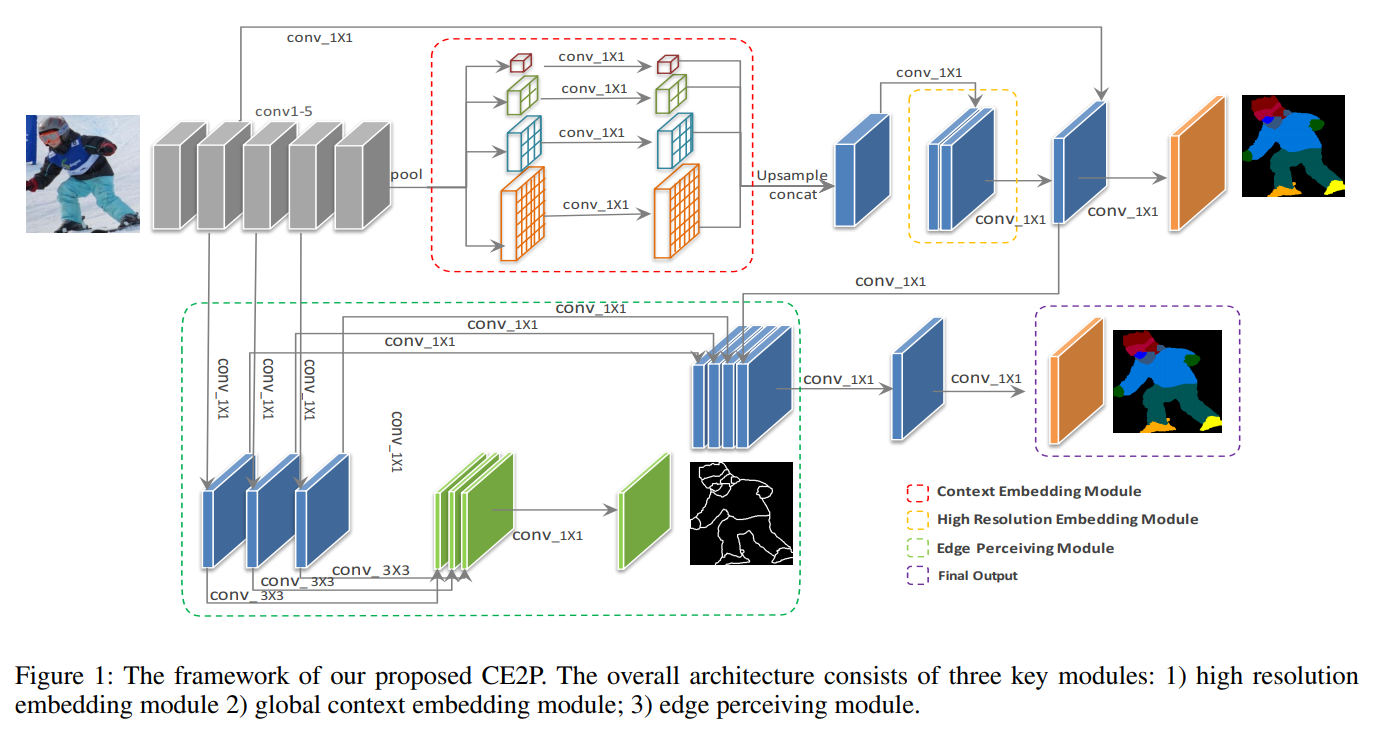
图中红色部分是PSPModule

class PSPModule(nn.Module):  # Pyramid scene parsing network
    """
    Reference: 
    Zhao, Hengshuang, et al. *"Pyramid scene parsing network."*
    """
    def __init__(self, features, out_features=512, sizes=(1, 2, 3, 6)):
        super(PSPModule, self).__init__()
        self.stages = []
        self.stages = nn.ModuleList([self._make_stage(features, out_features, size) for size in sizes])
        self.bottleneck = nn.Sequential(
            nn.Conv2d(features+len(sizes)*out_features, out_features, kernel_size=3, padding=1, dilation=1, bias=False),
            InPlaceABNSync(out_features),
            )
    def _make_stage(self, features, out_features, size):
        prior = nn.AdaptiveAvgPool2d(output_size=(size, size))
        conv = nn.Conv2d(features, out_features, kernel_size=1, bias=False)
        bn = InPlaceABNSync(out_features)
        return nn.Sequential(prior, conv, bn)
    def forward(self, feats):
        h, w = feats.size(2), feats.size(3)
        priors = [ F.interpolate(input=stage(feats), size=(h, w), mode='bilinear', align_corners=True) for stage in self.stages] + [feats]
        bottle = self.bottleneck(torch.cat(priors, 1))
        return bottle

黄色部分是 high-res 的module，常规的conv cat操作

class Decoder_Module(nn.Module):
    def __init__(self, num_classes):
        super(Decoder_Module, self).__init__()
        self.conv1 = nn.Sequential(
            nn.Conv2d(512, 256, kernel_size=1, padding=0, dilation=1, bias=False),
            InPlaceABNSync(256)
            )
        self.conv2 = nn.Sequential(
            nn.Conv2d(256, 48, kernel_size=1, stride=1, padding=0, dilation=1, bias=False),
            InPlaceABNSync(48)
            )
        self.conv3 = nn.Sequential(
            nn.Conv2d(304, 256, kernel_size=1, padding=0, dilation=1, bias=False),
            InPlaceABNSync(256),
            nn.Conv2d(256, 256, kernel_size=1, padding=0, dilation=1, bias=False),
            InPlaceABNSync(256)
            )
        self.conv4 = nn.Conv2d(256, num_classes, kernel_size=1, padding=0, dilation=1, bias=True)

    def forward(self, xt, xl):
        _, _, h, w = xl.size()

        xt = F.interpolate(self.conv1(xt), size=(h, w), mode='bilinear', align_corners=True)
        xl = self.conv2(xl)
        x = torch.cat([xt, xl], dim=1)
        x = self.conv3(x)
        seg = self.conv4(x)
        return seg, x

绿色部分是本文的亮点 Edge_Module，一方面提取了边缘特征信息，另一方面得到了edge图用于计算loss，从代码上看也是非常普通的做法

class Edge_Module(nn.Module):
    def __init__(self,in_fea=[256,512,1024], mid_fea=256, out_fea=2):
        super(Edge_Module, self).__init__()
        
        self.conv1 =  nn.Sequential(
            nn.Conv2d(in_fea[0], mid_fea, kernel_size=1, padding=0, dilation=1, bias=False),
            InPlaceABNSync(mid_fea)
            ) 
        self.conv2 =  nn.Sequential(
            nn.Conv2d(in_fea[1], mid_fea, kernel_size=1, padding=0, dilation=1, bias=False),
            InPlaceABNSync(mid_fea)
            )  
        self.conv3 =  nn.Sequential(
            nn.Conv2d(in_fea[2], mid_fea, kernel_size=1, padding=0, dilation=1, bias=False),
            InPlaceABNSync(mid_fea)
        )
        self.conv4 = nn.Conv2d(mid_fea,out_fea, kernel_size=3, padding=1, dilation=1, bias=True)
        self.conv5 = nn.Conv2d(out_fea*3,out_fea, kernel_size=1, padding=0, dilation=1, bias=True)

    def forward(self, x1, x2, x3):
        _, _, h, w = x1.size()
        
        edge1_fea = self.conv1(x1)
        edge1 = self.conv4(edge1_fea)
        edge2_fea = self.conv2(x2)
        edge2 = self.conv4(edge2_fea)
        edge3_fea = self.conv3(x3)
        edge3 = self.conv4(edge3_fea)        
        
        edge2_fea =  F.interpolate(edge2_fea, size=(h, w), mode='bilinear',align_corners=True) 
        edge3_fea =  F.interpolate(edge3_fea, size=(h, w), mode='bilinear',align_corners=True) 
        edge2 =  F.interpolate(edge2, size=(h, w), mode='bilinear',align_corners=True)
        edge3 =  F.interpolate(edge3, size=(h, w), mode='bilinear',align_corners=True) 
 
        edge = torch.cat([edge1, edge2, edge3], dim=1)
        edge = self.conv5(edge)

        edge_fea = torch.cat([edge1_fea, edge2_fea, edge3_fea], dim=1)

        return edge, edge_fea

Note that the edge annotation used in the edge perceiving module is directly generated from the parsing annotation by extracting border between different semantics.

仅是使用parsing的annotation，就生成了edge的annotation

def generate_edge(label, edge_width=3):
    h, w = label.shape
    edge = np.zeros(label.shape)    
    # right
    edge_right = edge[1:h, :]
        edge_right[(label[1:h, :] != label[:h - 1, :]) & (label[1:h, :] != 255)
                  & (label[:h - 1, :] != 255)] = 1  
    # up
    edge_up = edge[:, :w - 1]
        edge_up[(label[:, :w - 1] != label[:, 1:w])
               & (label[:, :w - 1] != 255)
               & (label[:, 1:w] != 255)] = 1    
    # upright
    edge_upright = edge[:h - 1, :w - 1]
        edge_upright[(label[:h - 1, :w - 1] != label[1:h, 1:w])
                    & (label[:h - 1, :w - 1] != 255)
                    & (label[1:h, 1:w] != 255)] = 1 
    # bottomright
    edge_bottomright = edge[:h - 1, 1:w]
        edge_bottomright[(label[:h - 1, 1:w] != label[1:h, :w - 1])
                        & (label[:h - 1, 1:w] != 255)
                        & (label[1:h, :w - 1] != 255)] = 1  
    kernel = cv2.getStructuringElement(cv2.MORPH_RECT, (edge_width, edge_width))
    edge = cv2.dilate(edge, kernel)
    return edge

LOSS
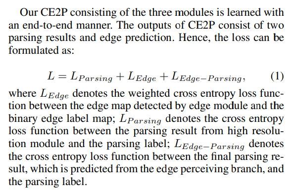
- CE三连
Experiment
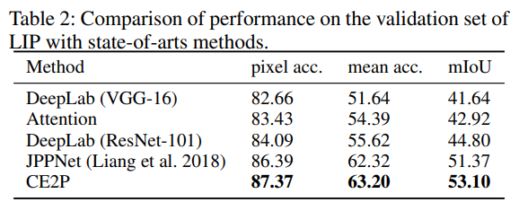
- 在不适用point的监督信息的情况下mIOU还提升了不少，比deeplab提升近9个点(20%)，在test集上，结果非常惊艳，远超JPP
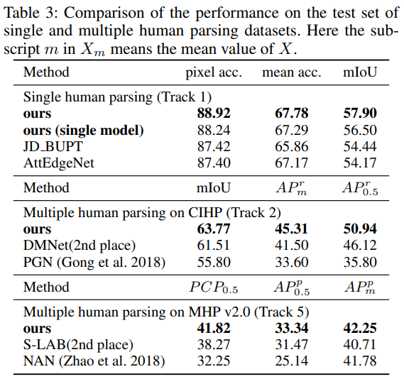
非常强大的结构，非常值得作为baseline使用

ACE2P-pp

git https://github.com/PaddlePaddle/PaddleSeg/tree/release/v0.1.0/contrib/ACE2P
目前的总统山榜首是 paddleseg 的 Augmented Context Embedding with Edge Perceiving(ACE2P)
ACE2P有两个版本，此处版本为rank 1的paddleseg版本，只有inference版本，paddlepaddle是静态图，具体信息的放出也比较有限
改编自 Devil in the Details: Towards Accurate Single and Multiple Human Parsing https://arxiv.org/abs/1809.05996
结构图
ACE2P模型包含三个分支:
1. 语义分割分支
2. 边缘检测分支
3. 融合分支
语义分割分支采用resnet101作为backbone,通过Pyramid Scene Parsing Network融合上下文信息以获得更加精确的特征表征
边缘检测分支采用backbone的中间层特征作为输入，预测二值边缘信息
融合分支将语义分割分支以及边缘检测分支的特征进行融合，以获得边缘细节更加准确的分割图像。
分割问题一般采用mIoU作为评价指标，特别引入了IoU loss结合cross-entropy loss以针对性优化这一指标
测试阶段，采用多尺度以及水平翻转的结果进行融合生成最终预测结果
训练阶段，采用余弦退火的学习率策略，并且在学习初始阶段采用线性warm up
数据预处理方面，保持图片比例并进行随机缩放，随机旋转，水平翻转作为数据增强策略
LIP指标
- 该模型在测试尺度为’377,377,473,473,567,567’且水平翻转的情况下，meanIoU为62.63
- 多模型ensemble后meanIoU为65.18, 居LIP Single-Person Human Parsing Track榜单第一
主要思想来自于 CE2P
和CE2P相比，几乎没有太多的变化，仅仅多了从 edge 分支到fuse分支一条线路
目前的LIP第一，使用paddlepaddle架构，放出了模型和推论脚本，没有训练脚本

ACE2P

paper Self-Correction for Human Parsing
该篇文章为ACE2P rank3版本，学术版本，10月22日首次挂在arxiv
git https://github.com/PeikeLi/Self-Correction-Human-Parsing
git版本只有inference，不过值得一提的是，由于使用的是pytorch，model是开放的可见的，对比ce2p后发现基本结构基本没有不同，区别在于loss和schp方法
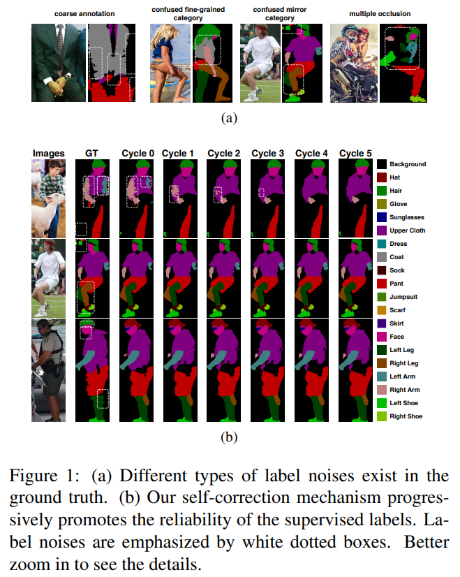
展示了schp随cycle改进pred的效果
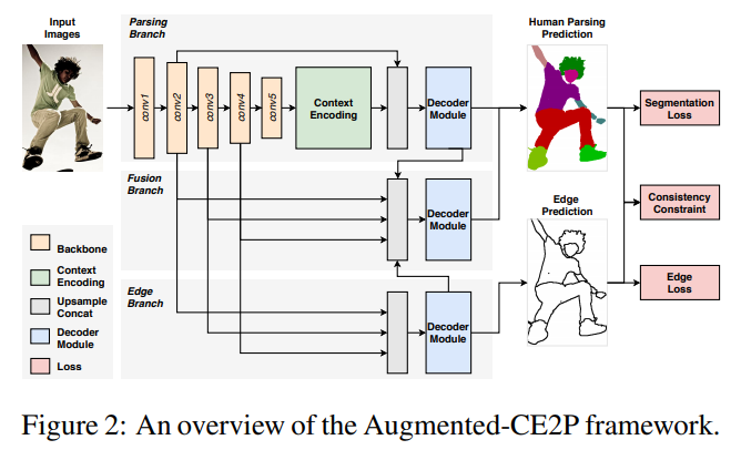
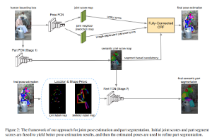
framework和paddleseg的基本一直，只是将loss function展开了，其中consistency constraint是一个新玩意。其中还有一点没有确定的是，ce2p是明显有三个输出的framework，这里的这个看样子仅有两个输出，有待实验确定
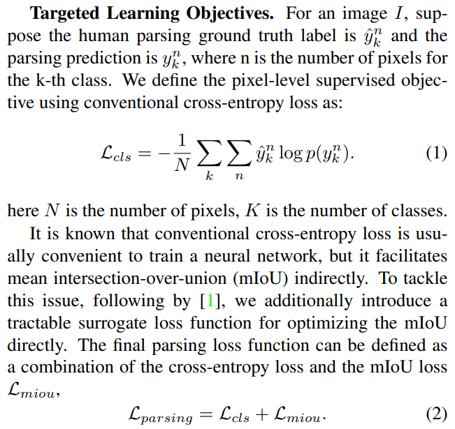
loss的第一部分是objective loss，是cls loss（bce） + miou loss。文中的[1] The Lovasz-Softmax loss: A tractable surrogate for the optimization of the ´ intersection-over-union measure in neural networks 是针对miou进行优化的loss，git https://github.com/bermanmaxim/LovaszSoftmax，有兴趣的同学可以点进去看看
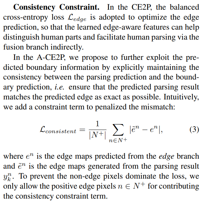
一致性约束。主要是为了回应他前文所说的
- Second, CE2P only implicitly facilitates the parsing results with the edge predictions by feature-level fusion. There is no explicit constraint to ensure the parsing results maintaining the same geometry shape of the boundary predictions.
这个edge module是否真的是帮助了pred，这里比对了pred中的edge和pred中fuse后gen出的edge，以保证这个fuse是靠谱的
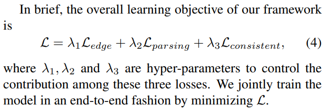
loss
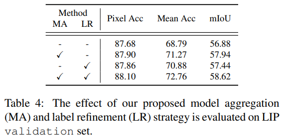
- We choose the ResNet-set. 101 [12] as the backbone of the feature extractor and use an ImageNet [8] pre-trained weights. Specifically, we fix the first three residual layers and set the stride size of last residual layer to 1 with a dilation rate of 2. In this way, the final output is enlarged to 1/16 resolution size w.r.t the original image. We adopt pyramid scene parsing network [33] as the context encoding module. We use 473 × 473 as the input resolution. Training is done with a total batch size of 36. For our joint loss function, we set the weight of each term as λ1 = 1, λ2 = 1, λ3 = 0.1. The initial learning rate is set as 7e-3 with a linear increasing warm-up strategy for 10 epochs. We train our network for 150 epochs in total for a fair comparison, the first 100 epochs as initialization following 5 cycles each contains 10 epochs of the self-correction process.
训练细节
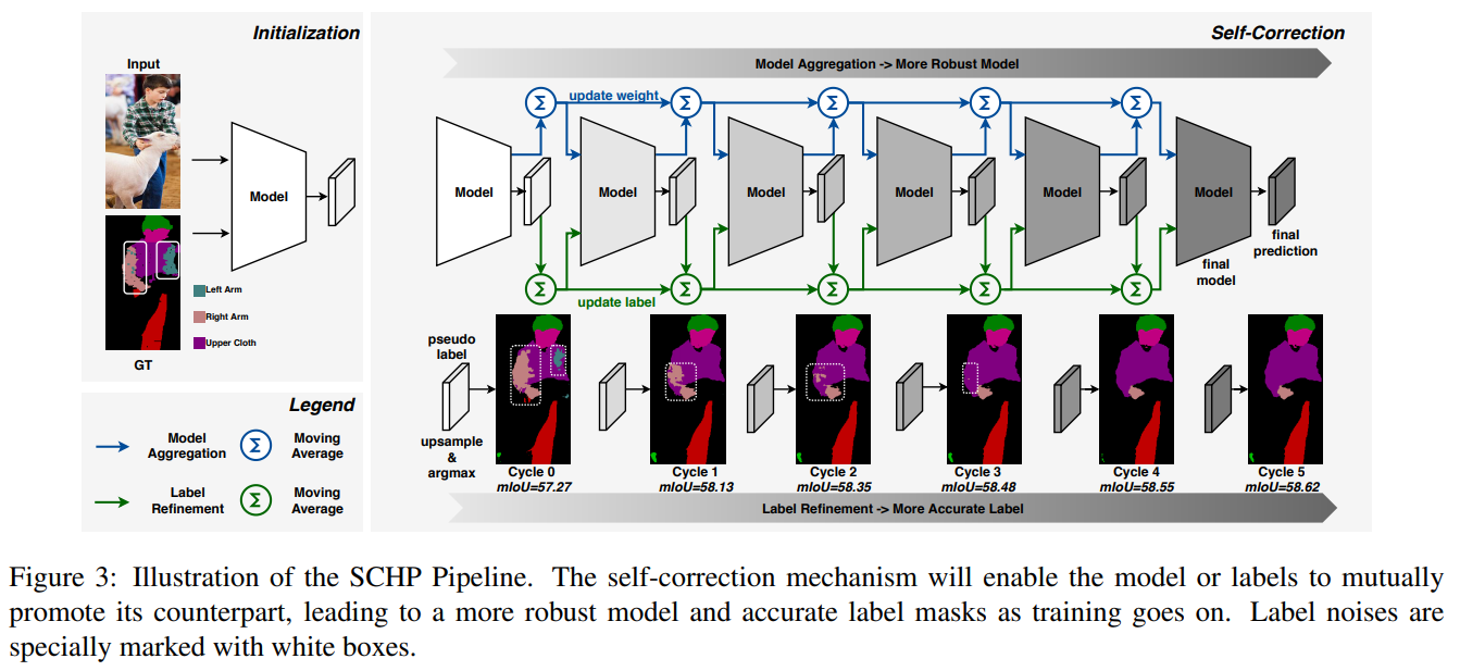
- 展示了schp的策略，先训练了100个epoch作为Cycle 0 base，然后使用 anneal cosine decay lr策略restart4次，将权重结合，模型效果就会像是ensemble了一样，越来越好
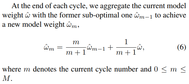
- 这个weight aggregation也是很直白的，w0是init的，m=1 w1 = m/(m+1) w0 + 1/(m+1)w = 1/2w0 + 1/2*w，就是一个移动平均
- After updating the current model weight with the former optimal one from the last cycle, we forward all the training data for one epoch to re-estimate the statistics of the parameters (i.e. moving average and standard deviation) in all batch normalization [14] layers. During these successive cycles of model aggregation, the network leads to wider model optima as well as improved model’s generalization ability.
- 作者也提到说模型融合的时候需要一个epoch来使BN层适应
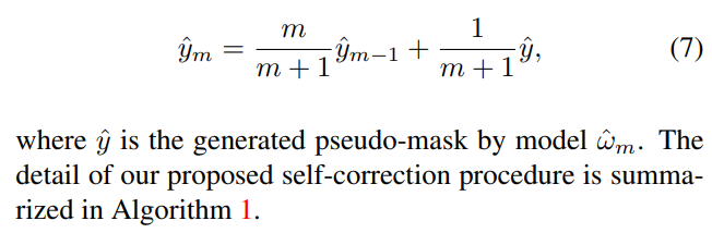
- 这个是说，怕这个label坑爹，使用原始的label init y0，使用pred结果更新label，机制和weight一样
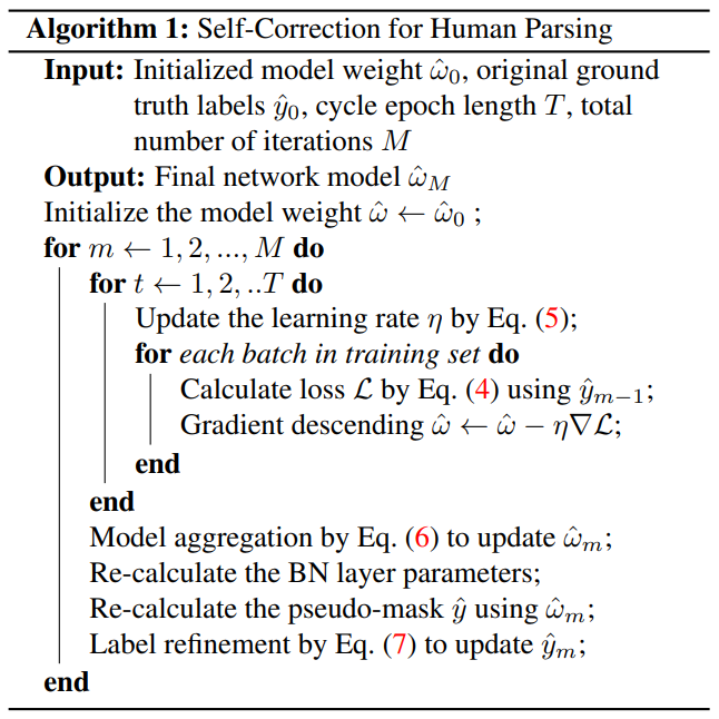
- schp的核心算法，每经过一次cycle，更新w，BN的parameter（mean var）不算w，额外更新下，使用新的w计算pred的y，更新y
Experiment
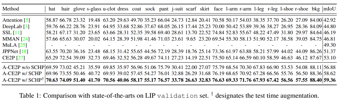
- ACE2P效果就很棒，加上SCHP，效果超CE2P一大截
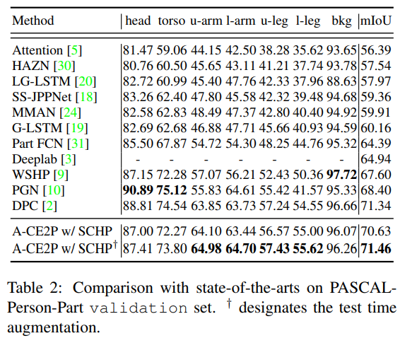
- 在 Pascal-Person-Part val上表现也同样不俗，使用简单的test技巧后达到了sota
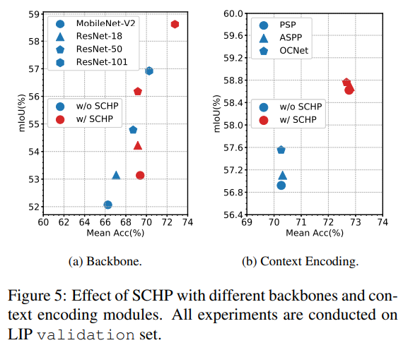
- 作者还在LIP上做了不同backbone的SCHP实验，使用SCHP能普涨一个点以上；当使用不同context encoding模块，使用了SCHP后，PSP ，ASPP，OCNet都得到了一个点以上的提升，差距缩小
- 说明了3个额外loss的可靠性；说明了schp中模型融合和label的refine都是有效果的
CE2P是正式在semantic segmentation中开启了human parsing分支，ACE2P是大幅改进了性能，都是非常推荐精读细读的文章

Dataset

LIP

look into person
home http://sysu-hcp.net/lip/overview.php
Human-Cyber-Physical Intelligence Integration Lab of Sun Yat-sen University （中山大学人机物智能融合实验室出品）
Overview
- Look into Person (LIP) is a new large-scale dataset, focus on semantic understanding of person. Following are the detailed descriptions.
  - Volume
    - The dataset contains 50,000 images with elaborated pixel-wise annotations with 19 semantic human part labels and 2D human poses with 16 key points.
  - Diversity
    - The annotated 50,000 images are cropped person instances from COCO dataset with size larger than 50 * 50.The images collected from the real-world scenarios contain human appearing with challenging poses and views, heavily occlusions, various appearances and low-resolutions. We are working on collecting and annotating more images to increase diversity.
Four Track
1. Single Person （Main）
  - We have divided images into three sets. 30462 images for training set, 10000 images for validation set and 10000 for testing set.The dataset is available at Google Drive and Baidu Drive.
  - Besides we have another large dataset mentioned in “Human parsing with contextualized convolutional neural network.” ICCV’15, which focuses on fashion images. You can download the dataset including 17000 images as extra training data.
2. Multi-Person (CHIP)
  - To stimulate the multiple-human parsing research, we collect the images with multiple person instances to establish the first standard and comprehensive benchmark for instance-level human parsing. Our Crowd Instance-level Human Parsing Dataset (CIHP) contains 28280 training, 5000 validation and 5000 test images, in which there are 38280 multiple-person images in total.
  - You can also downlod this dataset at Google Drive and Baidu Drive.
3. Video Multi-Person Human Parsing
  - VIP(Video instance-level Parsing) dataset, the first video multi-person human parsing benchmark, consists of 404 videos covering various scenarios. For every 25 consecutive frames in each video, one frame is annotated densely with pixel-wise semantic part categories and instance-level identification. There are 21247 densely annotated images in total. We divide these 404 sequences into 304 train sequences, 50 validation sequences and 50 test sequences.
  - You can also downlod this dataset at OneDrive and Baidu Drive.
    - VIP_Fine: All annotated images and fine annotations for train and val sets.
    - VIP_Sequence: 20-frame surrounding each VIP_Fine image (-10 | +10).
    - VIP_Videos: 404 video sequences of VIP dataset.
4. Image-based Multi-pose Virtual Try On
  - MPV (Multi-Pose Virtual try on) dataset, which consists of 35,687/13,524 person/clothes images, with the resolution of 256x192. Each person has different poses. We split them into the train/test set 52,236/10,544 three-tuples, respectively.

MHP

Multi-Human Parsing
home https://lv-mhp.github.io/
Learning and Vision (LV) Group, National University of Singapore (NUS) (新加坡国立大学机器学习与视觉小组)
Statistics
- MHP v1.0
  - The MHP v1.0 dataset contains 4,980 images, each with at least two persons (average is 3). We randomly choose 980 images and their corresponding annotations as the testing set. The rest form a training set of 3,000 images and a validation set of 1,000 images. For each instance, 18 semantic categories are defined and annotated except for the “background” category, i.e. “hat”, “hair”, “sunglasses”, “upper clothes”, “skirt”, “pants”, “dress”, “belt”, “left shoe”, “right shoe”, “face”, “left leg”, “right leg”, “left arm”, “right arm”, “bag”, “scarf” and “torso skin”. Each instance has a complete set of annotations whenever the corresponding category appears in the current image.
- MHP v2.0
  - The MHP v2.0 dataset contains 25,403 images, each with at least two persons (average is 3). We randomly choose 5,000 images and their corresponding annotations as the testing set. The rest form a training set of 15,403 images and a validation set of 5,000 images. For each instance, 58 semantic categories are defined and annotated except for the “background” category, i.e. “cap/hat”, “helmet”, “face”, “hair”, “left- arm”, “right-arm”, “left-hand”, “right-hand”, “protector”, “bikini/bra”, “jacket/windbreaker/hoodie”, “t-shirt”, “polo-shirt”, “sweater”, “sin- glet”, “torso-skin”, “pants”, “shorts/swim-shorts”, “skirt”, “stock- ings”, “socks”, “left-boot”, “right-boot”, “left-shoe”, “right-shoe”, “left- highheel”, “right-highheel”, “left-sandal”, “right-sandal”, “left-leg”, “right-leg”, “left-foot”, “right-foot”, “coat”, “dress”, “robe”, “jumpsuits”, “other-full-body-clothes”, “headwear”, “backpack”, “ball”, “bats”, “belt”, “bottle”, “carrybag”, “cases”, “sunglasses”, “eyewear”, “gloves”, “scarf”, “umbrella”, “wallet/purse”, “watch”, “wristband”, “tie”, “other-accessaries”, “other-upper-body-clothes”, and “other-lower-body-clothes”. Each instance has a complete set of annotations whenever the corresponding category appears in the current image.

Pascal-Person-Part Dataset

1,716 images for training and 1,817 for testing
first mentioned paper Detect What You Can: Detecting and Representing Objects using Holistic Models and Body Parts
- 没找到下载的地方= =。。标注了part
second paper Joint Multi-Person Pose Estimation and Semantic Part Segmentation
- download link
- 附加标注了key-point
- 提出了联合学习方法

ATR

project url link
paper Human Parsing with Contextualized Convolutional Neural Network
Human parsing is to predict every pixel with 18 labels: face, sunglass, hat, scarf, hair, upperclothes, left-arm, right-arm, belt, pants, left-leg, right-leg, skirt, left-shoe, right-shoe, bag, dress and null. Totally, 7,700 images are included in the ATR dataset [15], 6,000 for training, 1,000 for testing and 700 for validation1 . T
download link link